class: title-slide <br> <br> .right-panel[ <br> # Visualizing Data ## Dr. Mine Dogucu ] --- class: middle ## Reminder - Close all apps on your computer other than zoom. - Open slides for this session from the cluster website (https://uci-dshs.netlify.app/). --- class: middle ## Preparation 1. Please load the data named 'babies' from package named 'openintro' 2. Please install package named 'ggplot2' that used for visualization 3. Also, please load tidyverse in order to refresh data wrangling --- class: middle load data ``` r #install.packages('openintro') library(openintro) data("babies") ``` install ggplot2 ``` r #install.packages('ggplot2') library(ggplot2) ``` load tidyverse ``` r library(tidyverse) ``` --- class: middle ## Data ``` r glimpse(babies) ``` ``` ## Rows: 1,236 ## Columns: 8 ## $ case <int> 1, 2, 3, 4, 5, 6, 7, 8, 9, 10, 11, 12, 13, 14, 15, 16, 17, 1… ## $ bwt <int> 120, 113, 128, 123, 108, 136, 138, 132, 120, 143, 140, 144, … ## $ gestation <int> 284, 282, 279, NA, 282, 286, 244, 245, 289, 299, 351, 282, 2… ## $ parity <lgl> FALSE, FALSE, FALSE, FALSE, FALSE, FALSE, FALSE, FALSE, FALS… ## $ age <int> 27, 33, 28, 36, 23, 25, 33, 23, 25, 30, 27, 32, 23, 36, 30, … ## $ height <int> 62, 64, 64, 69, 67, 62, 62, 65, 62, 66, 68, 64, 63, 61, 63, … ## $ weight <int> 100, 135, 115, 190, 125, 93, 178, 140, 125, 136, 120, 124, 1… ## $ smoke <lgl> FALSE, FALSE, TRUE, FALSE, TRUE, FALSE, FALSE, FALSE, FALSE,… ``` --- class: middle __gg__plot is based on __g__rammar of __g__raphics. <!-- --> --- class:inverse middle .font75[Visualizing a Single Categorical Variable] --- class: middle .left-panel[ <br> <br> If you could speak to R in English, how would you tell R to make this plot for you? OR If you had the data and had to draw this bar plot by hand, what would you do? ] .right-panel[ <!-- --> ] --- class: middle .left-panel[ <br> <br> Possible ideas - Consider the data frame - Count number of babies for each type of mothers' `smoke` status - Put `smoke` on x-axis. - Put `count` on y-axis. - Draw the bars. ] .right-panel[ <!-- --> ] --- class: middle .left-panel[ <br> <br> These ideas are all correct but some are not necessary in R - Consider the data frame - ~~Count number of babies for each type of mothers' `smoke` status~~ - Put `smoke` on x-axis. - ~~Put `count` on y-axis.~~ - Draw the bars. R will do some of these steps by default. Making a bar plot with another tool might look slightly different. ] .right-panel[ <!-- --> ] --- class: middle **3 steps of making a basic ggplot** 1.Pick data 2.Map data onto aesthetics 3.Add the geometric layer --- class: middle ### Step 1 - Pick Data .pull-left[ ``` r ggplot(data = babies) ``` ] .pull-right[ <!-- --> ] --- class: middle ### Step 2 - Map Data to Aesthetics .pull-left[ ``` r ggplot(data = babies, * aes(x = smoke)) ``` ] .pull-right[ 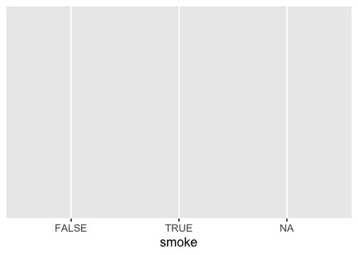<!-- --> ] --- class: middle ### Step 3 - Add the Geometric Layer .pull-left[ ``` r ggplot(data = babies, aes(x = smoke)) + * geom_bar() ``` ] .pull-right[ 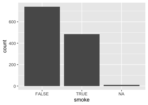<!-- --> ] --- class: middle .panelset[ .panel[ .panel-name[Plot] <img src="Lab-04a-visualize-data_files/figure-html/unnamed-chunk-16-1.png" style="display: block; margin: auto;" /> ] .panel[ .panel-name[English] - Create a ggplot using the `babies` data frame. - Map the `smoke` to the x-axis. - Add a layer of a bar plot. ] .panel[ .panel-name[R] ``` r ggplot(data = babies, aes(x = smoke)) + geom_bar() ``` ] ] --- class:inverse middle .font75[Visualizing a Single Numeric Variable] --- class: middle .panelset[ .panel[ .panel-name[Plot] ``` ## `stat_bin()` using `bins = 30`. Pick better value with `binwidth`. ``` <img src="Lab-04a-visualize-data_files/figure-html/unnamed-chunk-18-1.png" style="display: block; margin: auto;" /> ] .panel[ .panel-name[English] - Create a ggplot using the `babies` data frame. - Map the `bwt` to the x-axis. - Add a layer of a histogram. ] .panel[ .panel-name[R] ``` r ggplot(data = babies, aes(x = bwt)) + geom_histogram() ``` ] ] --- class: middle ### Step 1 - Pick Data .pull-left[ ``` r ggplot(data = babies) ``` ] .pull-right[ <!-- --> ] --- class: middle ### Step 2 - Map Data to Aesthetics .pull-left[ ``` r ggplot(data = babies, * aes(x = bwt)) ``` ] .pull-right[ 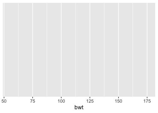<!-- --> ] --- class: middle ### Step 3 - Add the Geometric Layer .pull-left[ ``` r ggplot(data = babies, aes(x = bwt)) + * geom_histogram() ``` ] .pull-right[ ``` ## `stat_bin()` using `bins = 30`. Pick better value with `binwidth`. ``` 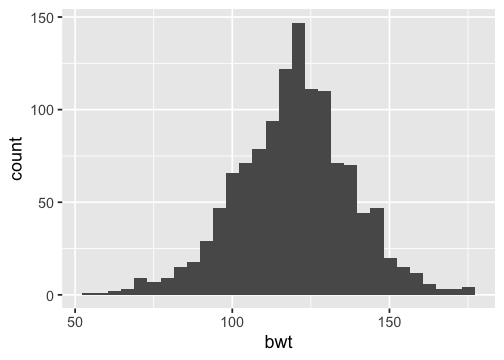<!-- --> ] --- ## What is this warning? ``` ## `stat_bin()` using `bins = 30`. Pick better value with `binwidth`. ``` <img src="Lab-04a-visualize-data_files/figure-html/unnamed-chunk-26-1.png" style="display: block; margin: auto;" /> --- ``` r ggplot(data = babies, aes(x = bwt)) + * geom_histogram(binwidth = 15) ``` <img src="Lab-04a-visualize-data_files/figure-html/unnamed-chunk-27-1.png" style="display: block; margin: auto;" /> --- class: middle .panelset[ .panel[.panel-name[binwidth = 15] .left-panel[ ] <img src="Lab-04a-visualize-data_files/figure-html/unnamed-chunk-28-1.png" style="display: block; margin: auto;" /> ] .panel[.panel-name[binwidth = 50] <img src="Lab-04a-visualize-data_files/figure-html/unnamed-chunk-29-1.png" style="display: block; margin: auto;" /> ] ] --- class: middle center Pick your favorite color(s) from the list at: [bit.ly/colors-r](https://bit.ly/colors-r) --- ``` r ggplot(data = babies, aes(x = bwt)) + geom_histogram(binwidth = 15, * color = "white") ``` <img src="Lab-04a-visualize-data_files/figure-html/unnamed-chunk-30-1.png" style="display: block; margin: auto;" /> --- ``` r ggplot(data = babies, aes(x = bwt)) + geom_histogram(binwidth = 15, * fill = "darkred") ``` <img src="Lab-04a-visualize-data_files/figure-html/unnamed-chunk-31-1.png" style="display: block; margin: auto;" /> --- ``` r ggplot(data = babies, aes(x = bwt)) + geom_histogram(binwidth = 15, * color = "white", * fill = "darkred") ``` <img src="Lab-04a-visualize-data_files/figure-html/unnamed-chunk-32-1.png" style="display: block; margin: auto;" /> --- class: inverse middle center .font75[Visualizing Two Categorical Variables] --- ## Stacked Bar-Plot .pull-left[ ``` r ggplot(data = babies, aes(x = smoke, * fill = parity)) + geom_bar() ``` ] .pull-right[ 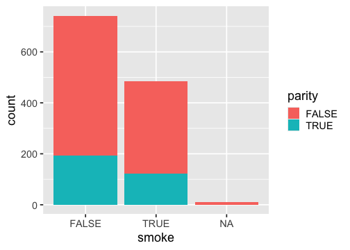<!-- --> ] --- ## Standardized Bar Plot .pull-left[ ``` r ggplot(data = babies, aes(x = smoke, fill = parity)) + * geom_bar(position = "fill") ``` ] .pull-right[ 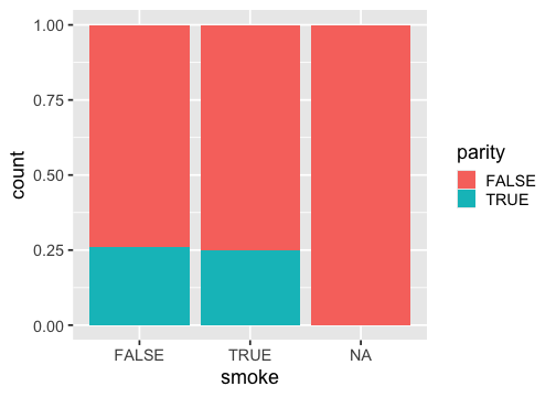<!-- --> ] .footnote[Note that y-axis is no longer count but we will learn how to change that later.] --- ## Dodged Bar Plot .pull-left[ ``` r ggplot(data = babies, aes(x = smoke, fill = parity)) + * geom_bar(position = "dodge") ``` ] .pull-right[ 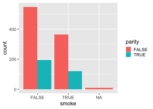<!-- --> ] .footnote[Note that y-axis is no longer count but we will change that later.] --- class: middle inverse .font75[Visualizing a single numerical and single categorical variable.] --- class: middle .panelset[ .panel[ .panel-name[Plot] <img src="Lab-04a-visualize-data_files/figure-html/unnamed-chunk-39-1.png" style="display: block; margin: auto;" /> ] .panel[ .panel-name[English] - Create a ggplot using the `babies` data frame. - Map the `smoke` to the x-axis and `bwt` to the y-axis. - Add a layer of a boxplot plot. ] .panel[ .panel-name[R] ``` r ggplot(babies, aes(x = smoke, y = bwt)) + geom_boxplot() ``` ] ] --- .pull-left[ 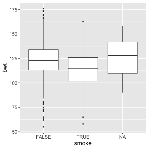<!-- --> ] .pull-right[ 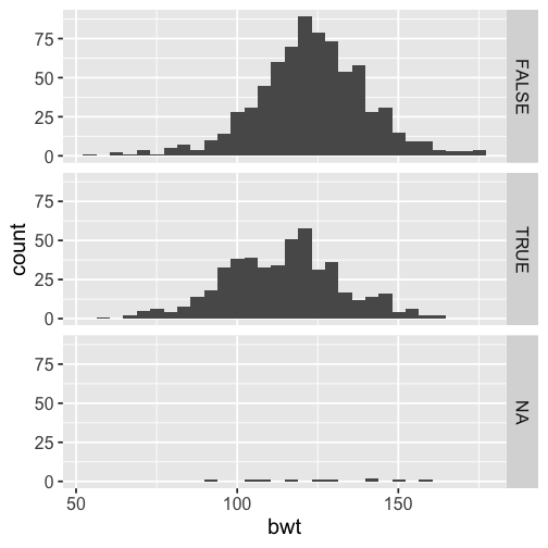<!-- --> ] --- class: inverse middle .font75[Visualizing Two Numerical Variables] --- .left-panel[ ``` r ggplot(babies, aes(x = gestation, y = bwt)) + geom_point() ``` ] .right-panel[ ``` ## Warning: Removed 13 rows containing missing values or values outside the scale range ## (`geom_point()`). ``` 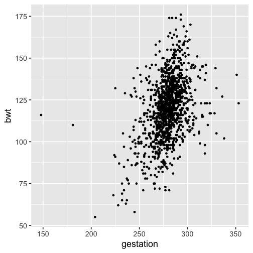<!-- --> ] --- class: middle inverse .font75[Considering More Than Two Variables] --- .left-panel[ ``` r ggplot(babies, aes(x = gestation, y = bwt, color = smoke)) + geom_point() ``` ] .right-panel[ ``` ## Warning: Removed 13 rows containing missing values or values outside the scale range ## (`geom_point()`). ``` 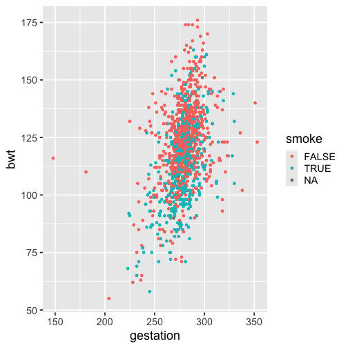<!-- --> ] --- .left-panel[ ``` r ggplot(babies, aes(x = gestation, y = bwt, shape = smoke)) + geom_point() ``` ] .right-panel[ ``` ## Warning: Removed 23 rows containing missing values or values outside the scale range ## (`geom_point()`). ``` <!-- --> ] --- .left-panel[ ``` r ggplot(babies, aes(x = gestation, y = bwt, shape = smoke)) + geom_point() ``` ] .right-panel[ ``` ## Warning: Removed 23 rows containing missing values or values outside the scale range ## (`geom_point()`). ``` 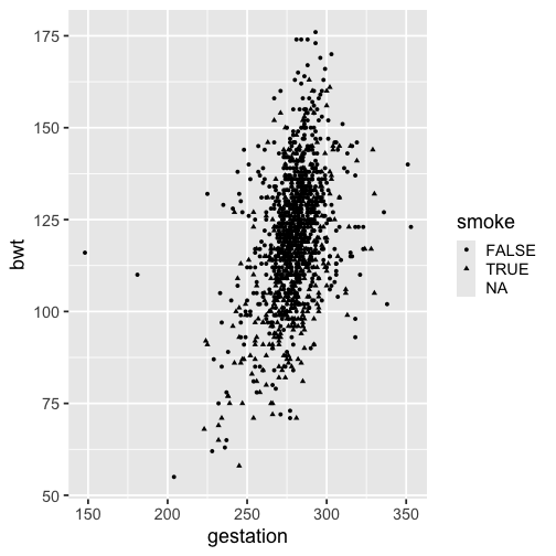<!-- --> ] --- .left-panel[ ``` r ggplot(babies, aes(x = gestation, y = bwt, shape = smoke, color = smoke)) + geom_point() ``` ] .right-panel[ ``` ## Warning: Removed 23 rows containing missing values or values outside the scale range ## (`geom_point()`). ``` 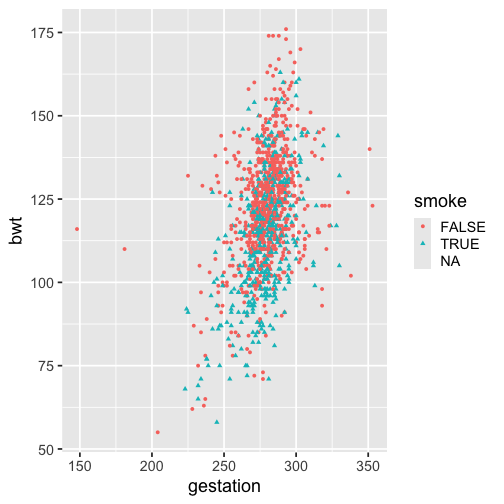<!-- --> ] --- .left-panel[ ``` r ggplot(babies, aes(x = gestation, y = bwt, shape = smoke, color = smoke, size = weight)) + geom_point() ``` ] .right-panel[ ``` ## Warning: Removed 58 rows containing missing values or values outside the scale range ## (`geom_point()`). ``` 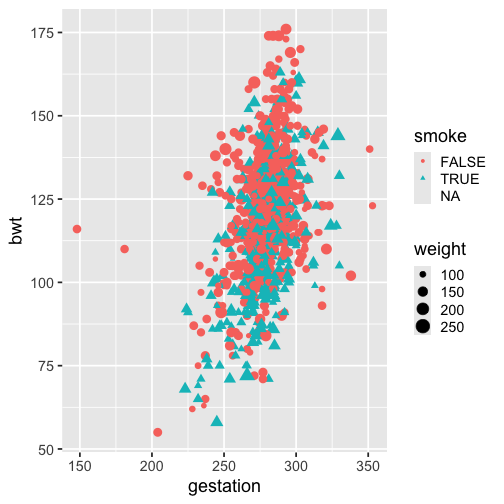<!-- --> ] --- <img src="img/ggplot-summary.jpeg" width="95%" />