Lab 1 intro to R

Data Science in Biomedical Sciences

UCI COSMOS 2026
Noah Benjamin
(adapted material from Sara Tyo and Mine Dogucu)

Slides

• Slides can be found on the website (https://cosmos-datascience.netlify.app).

First things first:

• Do you have a computer?
• Do you have R on your computer?
• Do you have RStudio on your computer?

Let’s talk about RStudio

Why is it a nice environment for R coding??

• It is an IDE(Integrated Development Environment) that we use to write, manage, and execute R code.

• It is open-source and free!! (and works well too)

• It’s not the only R-capable IDE, most of the popular ones have R extensions (like VSCode)

Today’s lab

We’re going to get some practice with the basics of R.

• The slides will walk through the concepts and serve as a reference. At the same time, we will each be writing the code on our computers to get some hands-on practice. I’ll also be doing it!!

• Please stop and ask questions!! It doesn’t have to just be if you’re stuck.

Creating a project in R studio

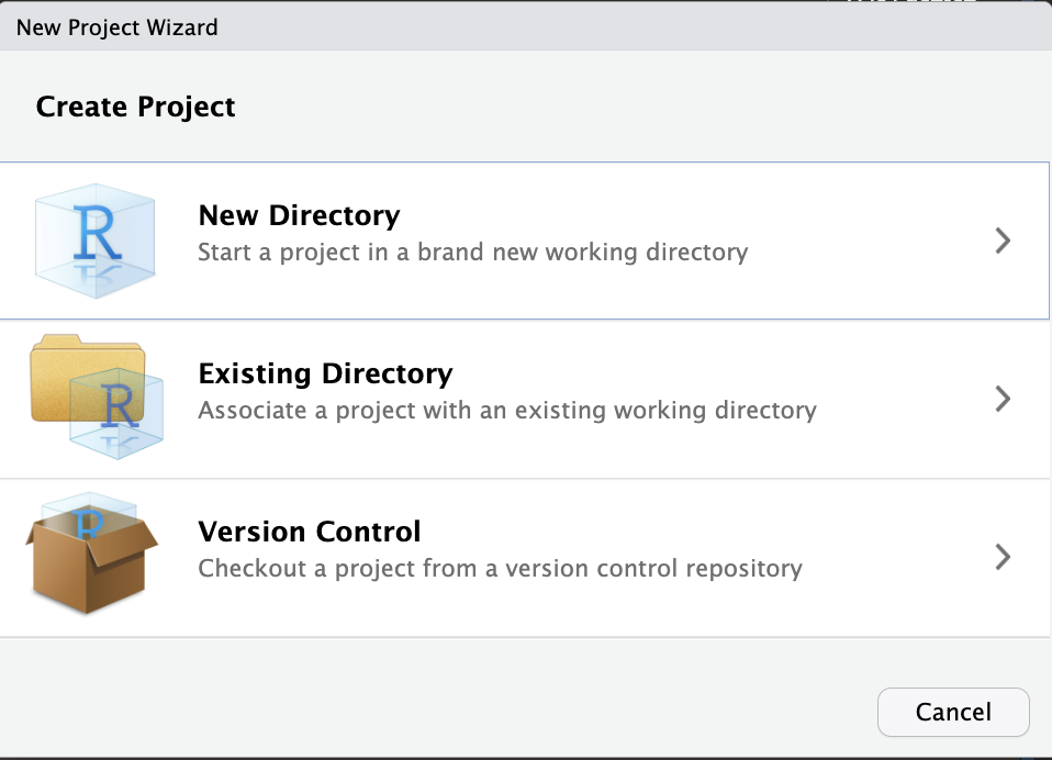
Create a new project

Creating a project in R studio

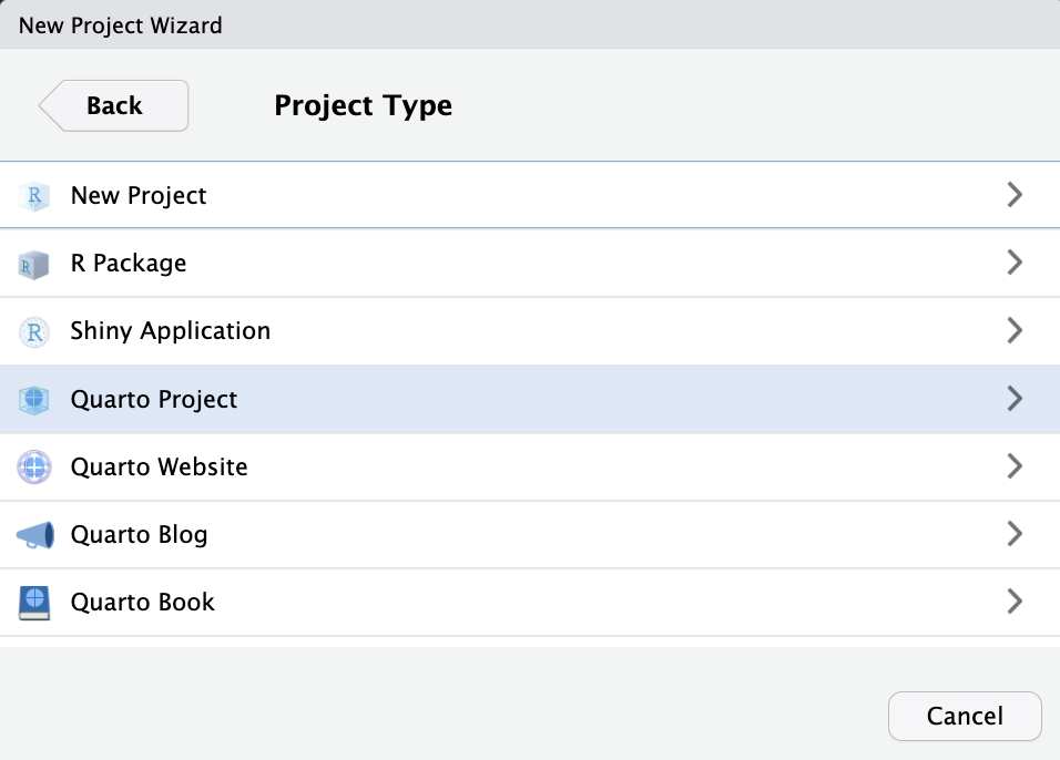
Choose a new Quarto project

Creating a project in R studio

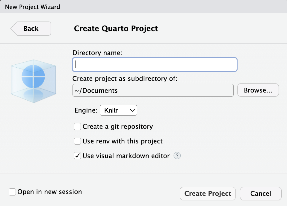
Create your new project!!

First, create a Quarto document

This is like a notebook file where you can write both text and code. It’s saved as a .qmd file.

• Quarto can run both R and Python!!! We will only be focusing on R.

• Also, it has built-in \(\LaTeX\) (very cool)

• \(y0u\mathbb{R}\varepsilon\) \(a\omega \varepsilon s0m\varepsilon\)

Lets start coding!

Code is written in code chunks:

# Hi I am a code chunk

Code chunks are delineated by

# Without the # mark:
# ```{r}
# ```

• To make a new code chunk, there is a handy keyboard shortcut

• (Ctrl + Alt + I)

• (Command + Option + I)

Math in R

• We can perform traditional mathematical operations in R

3+3 # add 3+3=6

[1] 6

4-1 # subtract 4-1=3

[1] 3

3/3 # divide 3/3=1

[1] 1

4*1 # multiply 4*1=4

[1] 4

2^4 # we can use either ^ or ** for exponent

[1] 16

2**4 

[1] 16

Math in R

• We can perform traditional mathematical operations in R

15 %% 2 # 'modulo', the remainder when (in this case) 15 is divided by 2

[1] 1

sqrt(16)

[1] 4

log(100)

[1] 4.60517

exp(4)

[1] 54.59815

Math in R

Try and write your own to solve:

\[\frac{e^4*|-ln(3)|}{-19*45}\]

(exp(4)*abs(-log(3)))/(-19*45)

[1] -0.07015462

Creating a variable (or object)

• The fancy term is the Assignment operator

• Basically just means we assign a value to a variable with the name we specify for it

birth_year <- 2000 # this is my birth year, maybe fill in your own!

• In this case we assigned the value 2000 to an object with the name birth_year

• We can then display the value of this variable by just running the variable name (either in it’s own chunk, or in the console)

birth_year

[1] 2000

Comments

• As you have already seen, we can write comments in our code chunks.

• We use the # symbol

• They are just for our reference and do not do anything when we run the chunk

• Like writing little notes in the code

my_age <- 2026 - birth_year # we can also do math in the code!!

R is case-sensitive

• Let’s say I want to display the variable I created on the previous slide

My_age

• R doesn’t like that because it’s very picky

• you can only reference the variable the exact way it was defined

my_age

[1] 26

Some other variable naming conventions/restrictions

Allowed Characters:

• letters (a-z, A-Z), numbers (0-9), dots (.), and underscores (_)

Forbidden Characters:

• spaces and some special characters (!, @, #, $, %, -)

Starting Character:

• variables names must start with a letter or a period (.)

• don’t start names with an underscore or a number

• can’t name a variable with a number right after a period (ex. .2var is invalid)

Variables in R

Variables are categorized into different types. You might be familiar with some of these already:

• character: takes string values (e.g. a person’s name, address)

• integer: integer (single precision)

• double: floating decimal (double precision)

• numeric: integer or double

• factor: categorical variables with different levels (ex. knitting skill: low, medium, high)

• logical: TRUE (1 or T), FALSE (0, or F)

Variables in R

If we have a variable we want to check the type of, we use the typeof() function.

typeof(1) # by default most numbers are stored as doubles

[1] "double"

typeof(1L) # using the L suffix forces R to store it as an integer

[1] "integer"

typeof(1.5)

[1] "double"

typeof(birth_year) # most of the time you will use typeof() on a variable like this

[1] "double"

typeof(as.integer(1))

[1] "integer"

A little more on character variables

• Anything we define in quotes is a string (even if it’s all numbers like “1234”).

• It’s how we differentiate variables names and text

"my_age" # is just the characters itself

[1] "my_age"

my_age # is the variable with the value we previously assigned to it

[1] 26

Vectors (or lists)

• Often, we want to store ordered lists of values, which we call vectors
• We call each component of the vector an element

• This is done using the c() function, which “concatenates” the values together into one vector

• Let’s create some vectors about fruit

fruits <- c("Apple", "Banana", "Orange")

colors <- c("red", "yellow", "orange")

seeds <- c(T, F, T)

Vectors (or lists)

• We can access specific elements in these vectors through indexing

• We index through the elements of a vector using the brackets []

• So, if we want to access the first element of the fruits vector we write:

fruits[1]

[1] "Apple"

• R is a 1-indexed language, meaning that when we index through a list we start at 1

• If you are familiar with Python, that is a 0-indexed language

data.frame

• One of the most common ways we will store data is in a data frame

• It’s like a spreadsheet, that stores data in a grid format

• In this grid each column (or row) is its own vector

• We can use our vectors about fruit to create a data.frame that stores all the info about fruit

fruit_data <- data.frame(fruit = fruits, color = colors, seeds = seeds)
fruit_data

   fruit  color seeds
1  Apple    red  TRUE
2 Banana yellow FALSE
3 Orange orange  TRUE

data.frame

• We can index the data.frame grid with brackets as well, indexing through the rows and columns

fruit_data[row, column]

fruit_data[2, 1] # this will give us the second row, first column entry of fruit_data

[1] "Banana"

• We can leave one of the row or column entries blank if we want the entire row or column

fruit_data[,1] # will give us the entire first column

[1] "Apple"  "Banana" "Orange"

fruit_data[3,] # will give us the entire third row

   fruit  color seeds
3 Orange orange  TRUE

Functions

• Let’s say we have a list of numbers, and we want to find the average of them

numbers <- c(-1, 15, 100, 111, 110)

• We could do this this mathematically, by adding up the values and dividing by how many there are

(-1 + 15 + 100 + 111 + 110)/5

[1] 67

Functions

• R has a lot of handy ways of making this quicker for us, however

• The sum() function will take the sum of the elements of the vector we pass into it
• The length() function will tell us how many elements are in the vector we give it

total <- sum(numbers)
how_many <- length(numbers)

total/how_many # so now we can find the mean this way

[1] 67

Functions

• Conveniently, R has a mean() function, which will do all of these things for us

mean(numbers)

[1] 67

Functions

Generally, we call functions in the following way:

do(something)

do() is a function;
something is the argument of the function.

Functions

Functions are not limited to only one argument:

do(something, colorful)

do() is a function;
something is the first argument of the function;
colorful is the second argument of the function.

• Some arguments might be optional, and start with default values

Functions

To learn about what a function does, we can use a question mark before the function:

?mean

• This will tell us what arguments a function expects, and default values for optional ones

Functions

• Many functions exist either in base R or in packages that save us from having to write our own code

• If you are looking for something specific, Google is your friend!!

• More on this coming up soon

Conditional statements

if(condition){
   Do Something
} else {
   Do Something Else
}

• We can add more conditions that are checked sequentially

Conditional statements

if(condition1){
  Do something
} else if (condition2) {
  Do a different thing
} else {
  Do this different thing
}

• Only one of the blocks will be run depending on which condition is met

Writing a condition

• == to check if something is equal (x == 2)

• != to check if it’s not equal to

Traditional inequalities also work: - <, >, <=, >=

Writing a condition

• We can also combine multiple conditions, to only execute if both conditions are met, or if one of two is met

• && check for both conditions to be true

• ex: if(x == 4 && y < 2), only returns TRUE if both conditions are met

• || checks for at least one of the conditions to be true

• ex: if(x == 4 || y < 2), returns TRUE if either of the two conditions are met

Conditional example 1

• Minimum height for rollercoaster

height <- 63
if(height >= 63){ # here we check if height is large enough to take the ride
  print("Fantastic! Enjoy the rollercoaster")
} else {
  print("OOPS! Sorry, you'll have to wait until next year")
}

[1] "Fantastic! Enjoy the rollercoaster"

Conditional example 2

• Whether to lend money, using logic in the condition

money <- 10
greed <- 1
if(money-1000 < 0 || greed > 50){ # here we check if we don't have enough money, or we are too greedy to lend
  print("Sorry I don't have enough money to loan you")
}else{
  print("Sure, here's 1000$.")
}

[1] "Sorry I don't have enough money to loan you"

Try and play around with the amount assigned to ‘money’ and ‘greed’.

Make your own

Now, Try and make your own if statement!

if(){
  print("")
}else{
  print("")
}

while loops and for loops

• while loops and for loops, as the names suggest repeat (or ‘loop’) a segment of code over and over

• a while loop runs code while a certain condition is met

• a for loop runs code for a pre-specified number of iterations

while loop syntax

while(condition) {
  Do this over and over 
}

• Be careful because its easy to write a while loop that runs for ever (and that is bad)

while loop example

x <- 0
while(x < 10) {
  x <- x + 1
}

• We can put any code we’d like in the loop

while loop example

x <- 0
while(x < 10) {
  x <- x + 1
  if(x %% 2 == 0) { # check if x is even
    print(x)
  }
}

[1] 2
[1] 4
[1] 6
[1] 8
[1] 10

while loop example

We can also forcibly break out of a loop when a certain condition is met, even if the loop has no actual end

x <- 1
while(TRUE) {
  if (x == 5) {
    break
  }
  print(x)
  x <- x + 1
}

[1] 1
[1] 2
[1] 3
[1] 4

for loop

• remember that for loops repeat for a specified number of iterations

• in the while loop example we just saw, we manually increased x by 1 every iteration of the loop

• for loops are special because they do this automatically

for loop syntax

for(element in vector){
  Do this as many times as there are elements in vector
}

• how this looks in practice:

for loop example

numbers <- c(1, 2, 3, 4, 5)
for(num in numbers) {
  print(num)
}

[1] 1
[1] 2
[1] 3
[1] 4
[1] 5

• one of the nice things about this is that the loop will iterate over any list, not just numbers

for loop example

for(fruit in fruits){ # using the fruits vector we defined earlier
  print(fruit)
}

[1] "Apple"
[1] "Banana"
[1] "Orange"

Creating Functions

Remember the length(), sum(), and mean() functions we saw earlier?

What if we want to make our own functions in R?

Writing your own functions is useful when you find you are rewriting the same code over and over again.

• We learned that functions take in arguments that are the user-inputted values when they call the function/

• The other indispensable ingredient in a function is a return() statement

• When a function hits return(some_value), it immediately ends and outputs the return value

Function syntax

Functions are made using the following syntax, where it’s important to prespecify the input arguments, and how you want them processed.

my_function <- function(input){
  if(input == TRUE){
    return("Fantastic!")
  }
  else{
    return("OOPS!")
  }
}

• What does this function take in, what are the arguments?

• What does this function do with those arguments?

What kind of inputs would return either result?

Running the function

When we run the my_function() code, we just created the function

• If we actually want to run it, we have to call it like we called the previous functions

ate_lunch <- TRUE
my_function(ate_lunch)

[1] "Fantastic!"

• We must first define the input variable, and then pass it into the function as an argument

Let’s write our own mean() function

my_mean <- function(numbers) {
  total <- sum(numbers)
  how_many <- length(numbers)
  return(total/numbers)
}

R packages

Sometimes, other people write functions that are useful to us. This is where packages come in.

A package is essentially a library of functions written by someone and compiled for a specific purpose

We use packages by first installing them, and then loading them into our R environment

R packages

Let’s ry running the following code:

beep()

Why are we seeing an error?

Answer: We don’t have this package downloaded.

Think of packages as items, when we have an error it means we have yet to get/purchase an item.

Installing ‘Getting’ a Package

You can copy or type install.packages(“beepr”) in the console, or in the a code chunk.

NOTE: we only ever need to install a package once. Once downloaded, we can ‘call’ it and use it whenever we want.

install.packages("beepr")

We can also use the ‘packages’ search in the bottom-right pane

Using Packages and Functions from Packages

We want to use the beep() function from the beepr package. So we first need to call/open the package.

How do we get it?

We use the function library() to recall and load in the package into our R session.

library("beepr")

Now try and run beep()

beep()

YAY!

We can still use ? to get help about a function

What if we want a different sound? Where do we go again if we don’t know what to do, or maybe want to learn more about a particular function?

Use help search bar, or ‘?’

?beep

Good packages have documentation written about what the functions do

We can still use ? to get help about a function

What kinds of sounds are there from the description?

• 1. ping

• 2…

• 3…

• Try out different sound types

beep(sound="wilhelm")

More Fun

Now, use the say() function from the library cowsay and see what it does

install.packages("cowsay")
library(cowsay)

Need Help?

?say()

• It will Print out default “Hello world”, and generate an image of a cat
• we can change what it says by adjusting the ‘what’ argument
• we can change the animal by adjusting the ‘by’ argument

What are some of the animals it can generate?

Are there other things you can change?

Play around!

say(what="Have Fun!", by="cat", what_color="green")