Code
    n  df  X90.  X95.  X99.
1 Inf Inf 1.645 1.960 2.576
2   5   4 2.132 2.776 4.604
3  10   9 1.833 2.262 3.250
4  20  19 1.729 2.093 2.861
5  50  49 1.677 2.010 2.680
6 100  99 1.660 1.984 2.626
Zhaoxia Yu
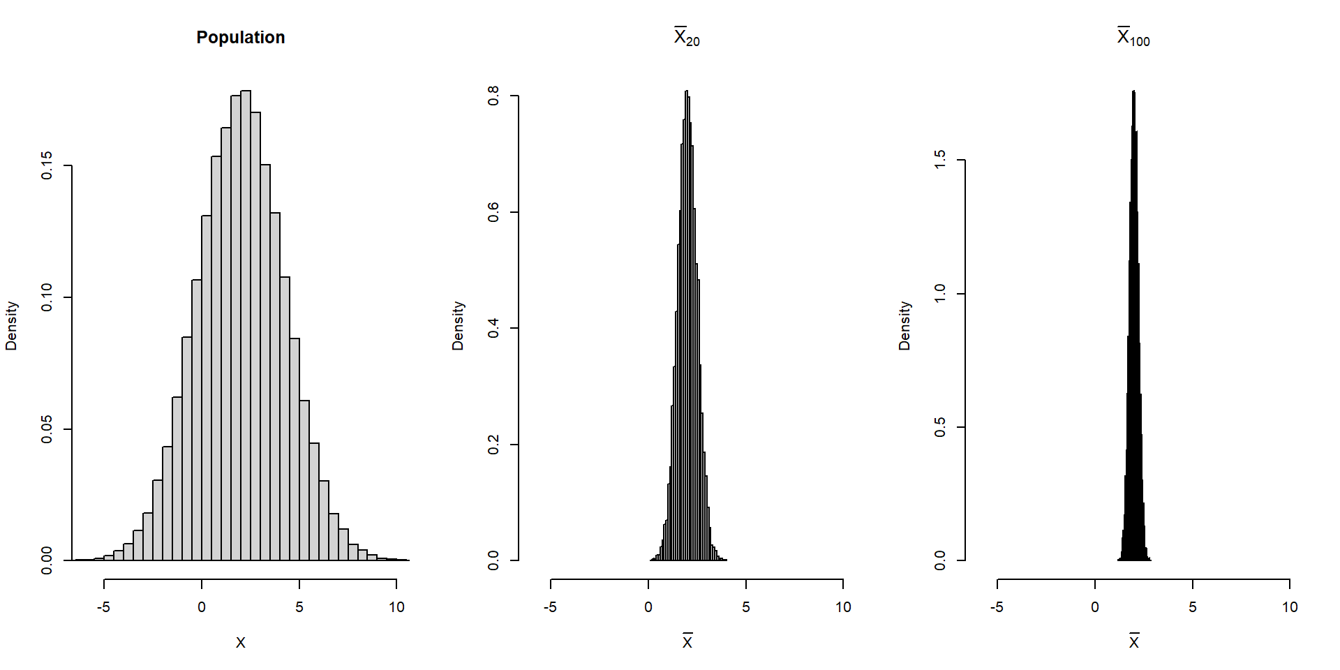
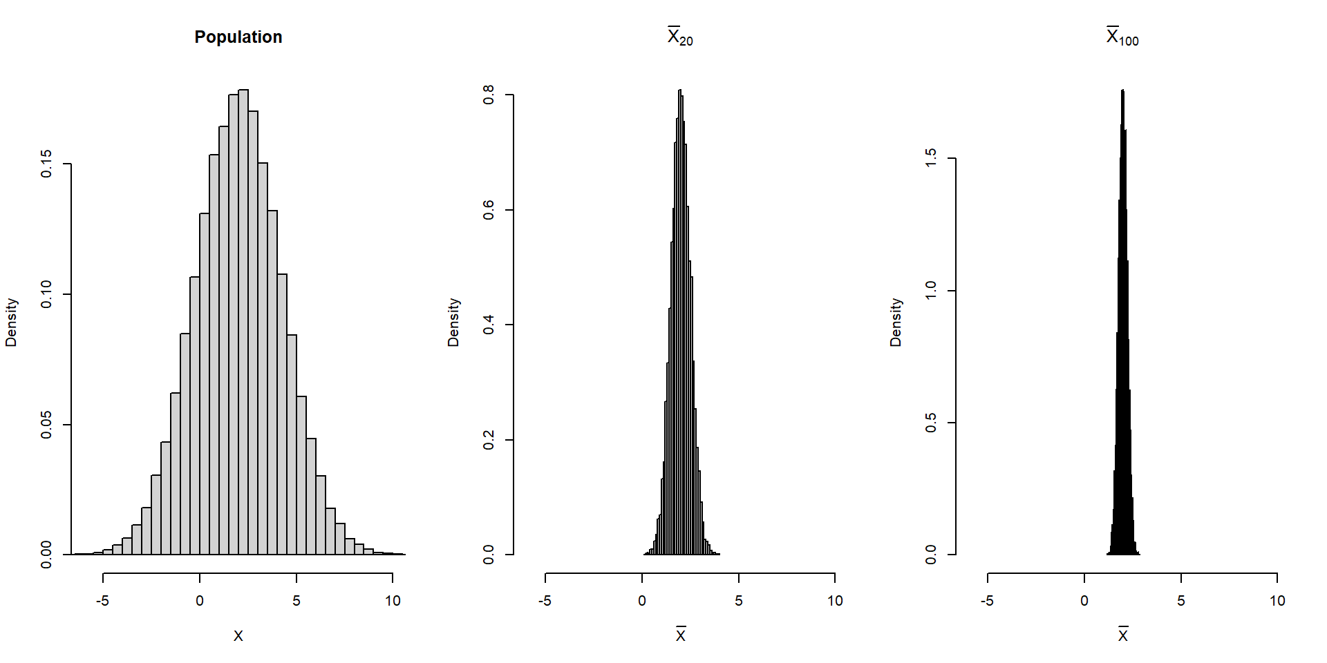
Suppose he population follows \(X\sim N(2,5).\)
\(\bar X_n\) also follows a normal distribution. Compare \(\bar X_{20}\) and \(\bar X_{100}\).
set.seed(20260709)

B <- 10000

# Population
x <- rnorm(100000, mean = 2, sd = sqrt(5))

# Sampling distributions
xbar20 <- replicate(B, mean(rnorm(20, mean = 2, sd = sqrt(5))))
xbar100 <- replicate(B, mean(rnorm(100, mean = 2, sd = sqrt(5))))

par(mfrow = c(1,3))

hist(x,
     probability = TRUE,
     breaks = 40,
     main = "Population",
     xlab = "X",
     xlim = c(-6,10))

hist(xbar20,
     probability = TRUE,
     breaks = 40,
     main = expression(bar(X)[20]),
     xlab = expression(bar(X)),
     xlim = c(-6,10))

hist(xbar100,
     probability = TRUE,
     breaks = 40,
     main = expression(bar(X)[100]),
     xlab = expression(bar(X)),
xlim = c(-6,10))library(tidyverse)
alzheimer_data <- read.csv("https://raw.githubusercontent.com/COSMOS-DataScience/slides/refs/heads/main/data/alzheimer_data.csv", head=T)%>%
select(id, diagnosis, age, educ, female, height, weight) %>%
mutate(diagnosis = as.factor(diagnosis), female = as.factor(female))
# Heights of female participants
f_height = alzheimer_data %>%
filter(female == 1) %>%
pull(height)
# histogram height of female
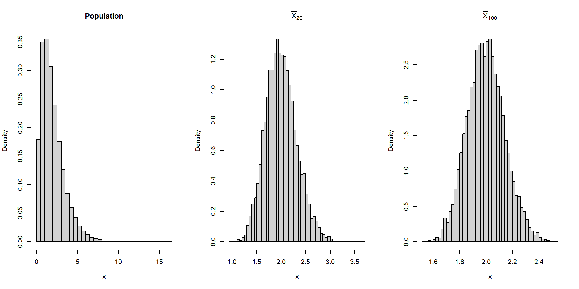
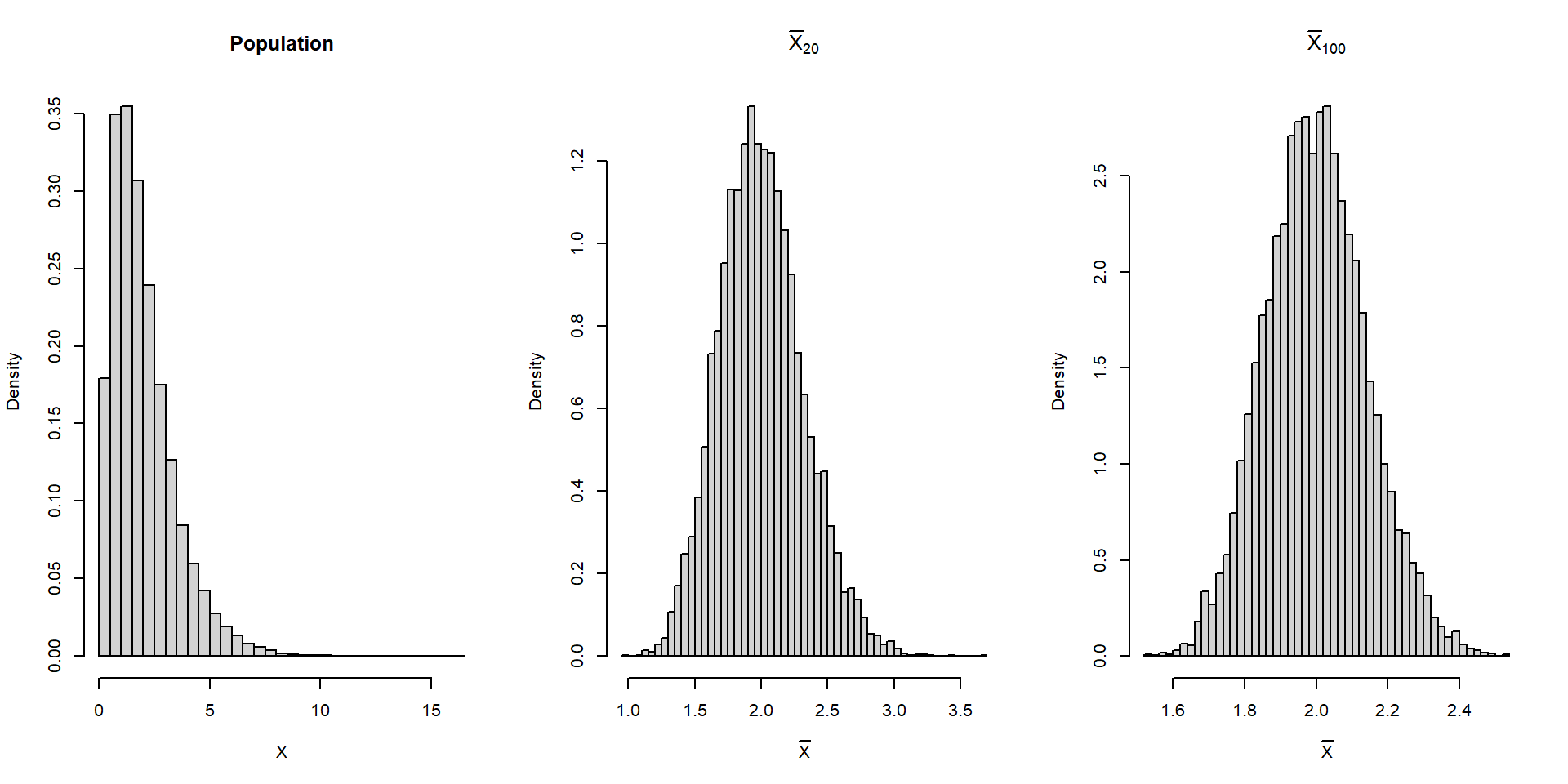
hist(f_height)Suppose the population is not normal, e.g., skewed.
Although the population is not normal, the sampling distribution of \(\bar X_n\) becomes approximately normal as the sample size increases.
set.seed(20260709)

B <- 10000

# Population
x <- rgamma(100000, shape = 2, scale = 1)

# Sampling distributions
xbar20 <- replicate(B, mean(rgamma(20, shape = 2, scale = 1)))
xbar100 <- replicate(B, mean(rgamma(100, shape = 2, scale = 1)))

par(mfrow = c(1,3))

hist(x,
     probability = TRUE,
     breaks = 40,
     main = "Population",
     xlab = "X")

hist(xbar20,
     probability = TRUE,
     breaks = 40,
     main = expression(bar(X)[20]),
     xlab = expression(bar(X)))

hist(xbar100,
     probability = TRUE,
     breaks = 40,
     main = expression(bar(X)[100]),
xlab = expression(bar(X)))set.seed(20260706)
p <- runif(1)
p_hat_all_sim1=rep(NA, 29)
for(i in 1:29){
set.seed(i)
x <- rbinom(n=10, 1, p)
p_hat_all_sim1[i] <- mean(x)
#print("Student ID: ", i, " p_hat: ", p_hat)
}
n=10
hist(p_hat_all_sim1, main="Distribution of p_hat for n=10", xlab="p_hat",
probability = TRUE, col="lightblue", border="black",
breaks = seq(-0.5/n, max(p_hat_all_sim1) + 0.5/n, by = 1/n))set.seed(20260706)
p <- runif(1)
p_hat_all_sim2=rep(NA, 29)
for(i in 1:29){
set.seed(i)
x <- rbinom(n=100, 1, p)
p_hat_all_sim2[i] <- mean(x)
#print("Student ID: ", i, " p_hat: ", p_hat)
}
n=100
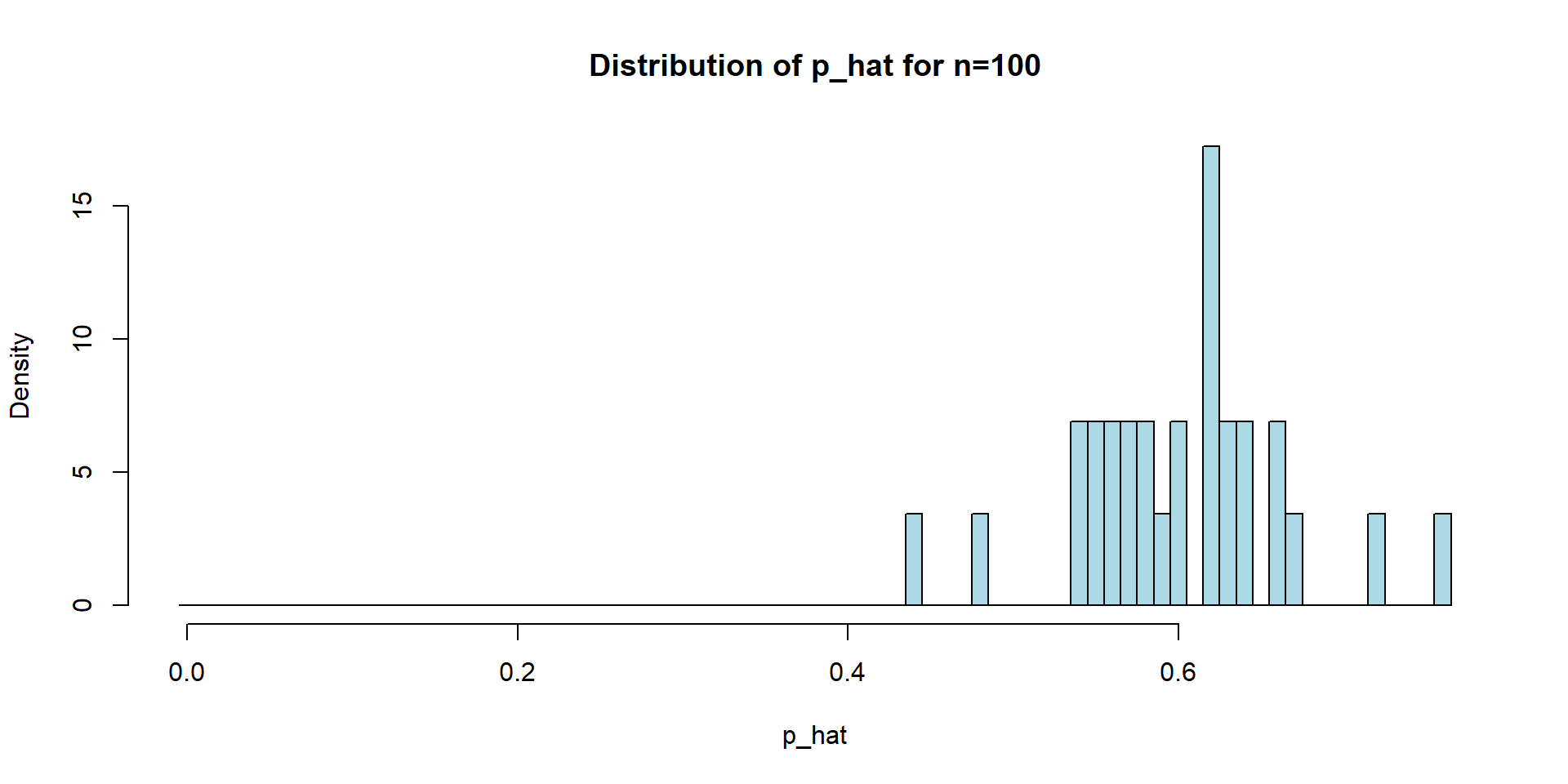
hist(p_hat_all_sim2, main="Distribution of p_hat for n=100", xlab="p_hat", probability = TRUE, col="lightblue", border="black",
breaks = seq(-0.5/n, max(p_hat_all_sim2) + 0.5/n, by = 1/n))par(mfrow=c(1,2))
n=10
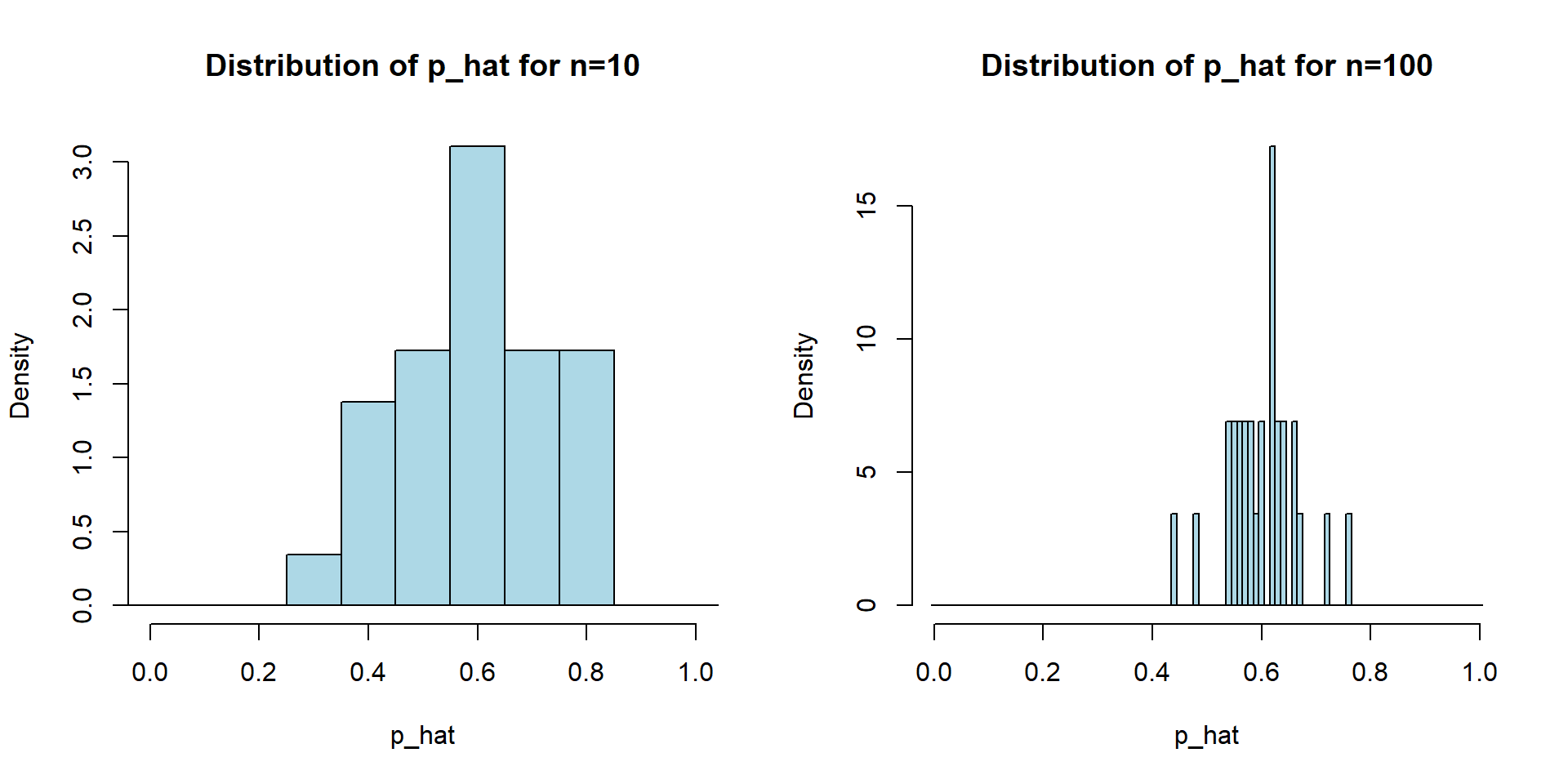
hist(p_hat_all_sim1, main="Distribution of p_hat for n=10", xlab="p_hat", probability = TRUE, col="lightblue", border="black", xlim=c(0,1),
breaks = seq(-0.5/n, 1 + 0.5/n, by = 1/n))
n=100
hist(p_hat_all_sim2, main="Distribution of p_hat for n=100", xlab="p_hat", probability = TRUE, col="lightblue", border="black", xlim=c(0,1),
breaks = seq(-0.5/n, 1 + 0.5/n, by = 1/n))# Number of simulated students
B <- 10000
# True probability (hidden)
set.seed(20260706)
p <- runif(1)
# Repeat the experiment B times
# for a large B, for loop is slow
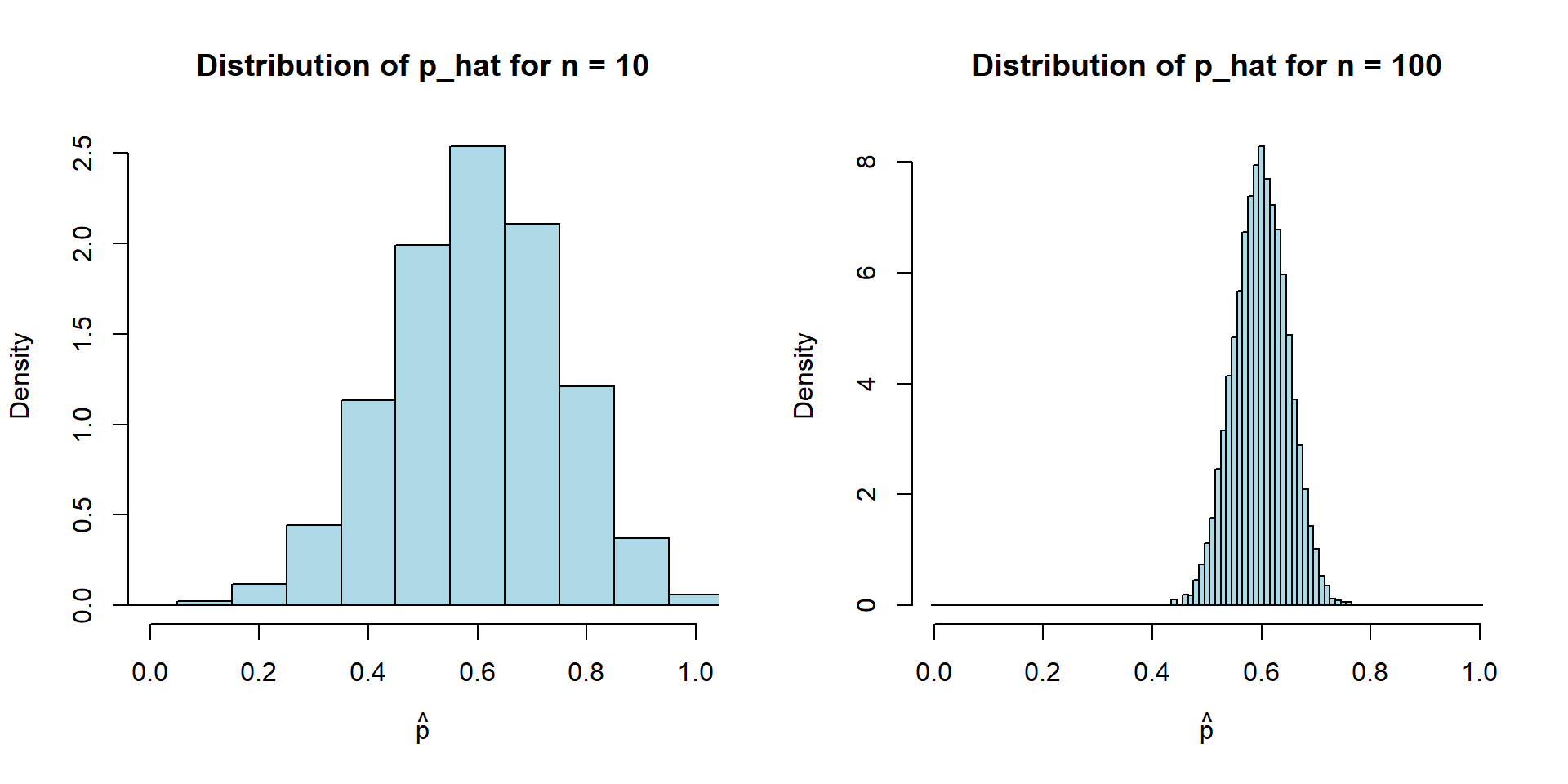
p_hat_all_sim1 <- replicate(B,
mean(rbinom(10, size = 1, prob = p)))
p_hat_all_sim2 <- replicate(B,
mean(rbinom(100, size = 1, prob = p)))
par(mfrow=c(1,2))
n <- 10
hist(
p_hat_all_sim1,
probability = TRUE,
breaks = seq(-0.5/n, 1 + 0.5/n, by = 1/n),
main = paste("Distribution of p_hat for n =", n),
xlab = expression(hat(p)),
col = "lightblue",
border = "black",
xlim = c(0, 1)
)
n <- 100
hist(
p_hat_all_sim2,
probability = TRUE,
breaks = seq(-0.5/n, 1 + 0.5/n, by = 1/n),
main = paste("Distribution of p_hat for n =", n),
xlab = expression(hat(p)),
col = "lightblue",
border = "black",
xlim = c(0, 1)
)# Number of simulated students
B <- 10000
# True probability (hidden)
set.seed(20260706)
p <- runif(1)
# Repeat the experiment B times
# for a large B, for loop is slow
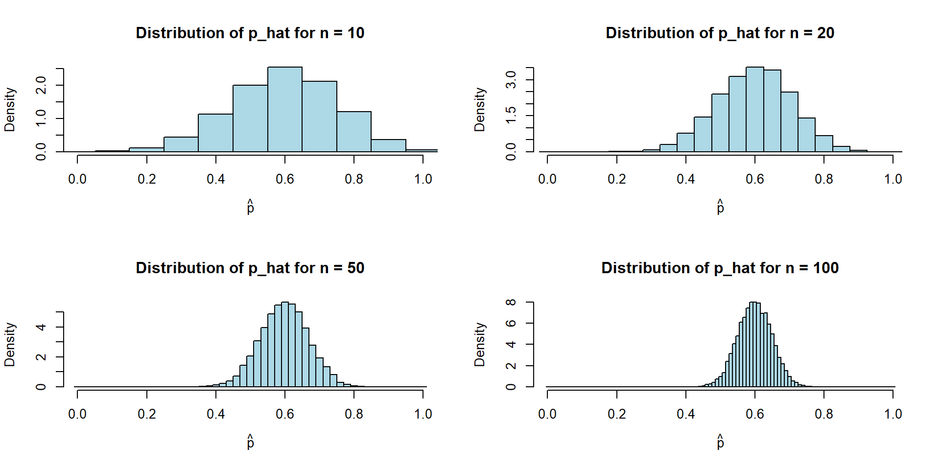
p_hat_all_sim10 <- replicate(B,
mean(rbinom(10, size = 1, prob = p)))
p_hat_all_sim20 <- replicate(B,
mean(rbinom(20, size = 1, prob = p)))
p_hat_all_sim50 <- replicate(B,
mean(rbinom(50, size = 1, prob = p)))
p_hat_all_sim100 <- replicate(B,
mean(rbinom(100, size = 1, prob = p)))
par(mfrow=c(2,2))
n <- 10
hist(
p_hat_all_sim10,
breaks = seq(-0.5/n, 1 + 0.5/n, by = 1/n),
probability = TRUE,
main = paste("Distribution of p_hat for n =", n),
xlab = expression(hat(p)),
col = "lightblue",
border = "black",
xlim = c(0, 1))
n <- 20
hist(
p_hat_all_sim20,
breaks = seq(-0.5/n, 1 + 0.5/n, by = 1/n),
probability = TRUE,
main = paste("Distribution of p_hat for n =", n),
xlab = expression(hat(p)),
col = "lightblue",
border = "black",
xlim = c(0, 1))
n <- 50
hist(
p_hat_all_sim50,
breaks = seq(-0.5/n, 1 + 0.5/n, by = 1/n),
probability = TRUE,
main = paste("Distribution of p_hat for n =", n),
xlab = expression(hat(p)),
col = "lightblue",
border = "black",
xlim = c(0, 1))
n <- 100
hist(
p_hat_all_sim100,
breaks = seq(-0.5/n, 1 + 0.5/n, by = 1/n),
probability = TRUE,
main = paste("Distribution of p_hat for n =", n),
xlab = expression(hat(p)),
col = "lightblue",
border = "black",
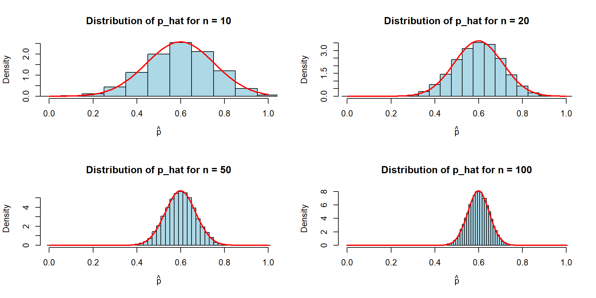
xlim = c(0, 1))par(mfrow=c(2,2))
n <- 10
hist(
p_hat_all_sim10,
breaks = seq(-0.5/n, 1 + 0.5/n, by = 1/n),
probability = TRUE,
main = paste("Distribution of p_hat for n =", n),
xlab = expression(hat(p)),
col = "lightblue",
border = "black",
xlim = c(0, 1))
curve(
dnorm(x, mean = p, sd = sqrt(p * (1 - p) / n)),
add = TRUE,
col = "red",
lwd = 2)
n <- 20
hist(
p_hat_all_sim20,
breaks = seq(-0.5/n, 1 + 0.5/n, by = 1/n),
probability = TRUE,
main = paste("Distribution of p_hat for n =", n),
xlab = expression(hat(p)),
col = "lightblue",
border = "black",
xlim = c(0, 1))
curve(
dnorm(x, mean = p, sd = sqrt(p * (1 - p) / n)),
add = TRUE,
col = "red",
lwd = 2)
n <- 50
hist(
p_hat_all_sim50,
breaks = seq(-0.5/n, 1 + 0.5/n, by = 1/n),
probability = TRUE,
main = paste("Distribution of p_hat for n =", n),
xlab = expression(hat(p)),
col = "lightblue",
border = "black",
xlim = c(0, 1))
curve(
dnorm(x, mean = p, sd = sqrt(p * (1 - p) / n)),
add = TRUE,
col = "red",
lwd = 2)
n <- 100
hist(
p_hat_all_sim100,
breaks = seq(-0.5/n, 1 + 0.5/n, by = 1/n),
probability = TRUE,
main = paste("Distribution of p_hat for n =", n),
xlab = expression(hat(p)),
col = "lightblue",
border = "black",
xlim = c(0, 1))
curve(
dnorm(x, mean = p, sd = sqrt(p * (1 - p) / n)),
add = TRUE,
col = "red",
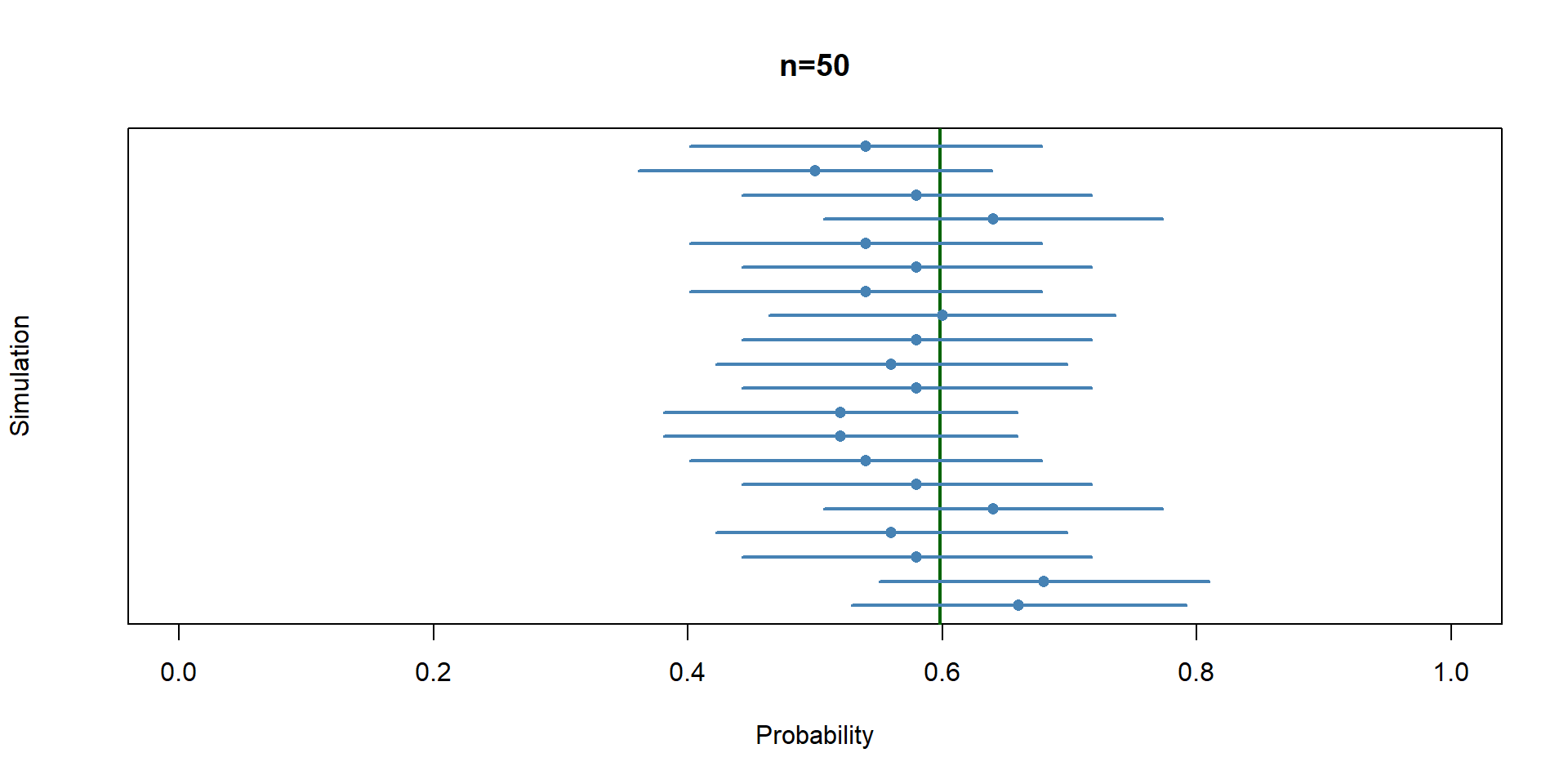
lwd = 2)B_show <- 20
plot(
NA,
xlim = c(0, 1),
ylim = c(1, B_show),
xlab = "Probability",
ylab = "Simulation",
yaxt = "n",
main="n=50"
)
abline(v = p, col = "darkgreen", lwd = 2)
for(i in 1:B_show){
col <- ifelse(cover[i], "steelblue", "red")
segments(lower[i], i, upper[i], i,
col = col, lwd = 2)
points(p_hat_all_sim50[i], i,
pch = 16,
col = col)
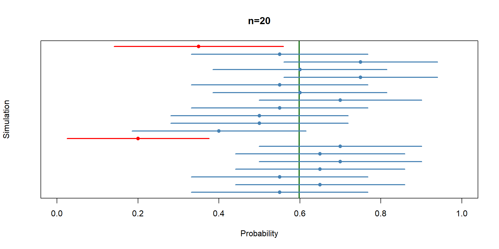
}B_show <- 20
plot(
NA,
xlim = c(0, 1),
ylim = c(1, B_show),
xlab = "Probability",
ylab = "Simulation",
yaxt = "n",
main="n=20"
)
abline(v = p, col = "darkgreen", lwd = 2)
for(i in 1:B_show){
col <- ifelse(cover[i], "steelblue", "red")
segments(lower[i], i, upper[i], i,
col = col, lwd = 2)
points(p_hat_all_sim20[i], i,
pch = 16,
col = col)
}Suppose he population follows \(X\sim N(2,5).\)
\(\bar X_n\) also follows a normal distribution. Compare \(\bar X_{20}\) and \(\bar X_{100}\).
set.seed(20260709)

B <- 10000

# Population
x <- rnorm(100000, mean = 2, sd = sqrt(5))

# Sampling distributions
xbar20 <- replicate(B, mean(rnorm(20, mean = 2, sd = sqrt(5))))
xbar100 <- replicate(B, mean(rnorm(100, mean = 2, sd = sqrt(5))))

par(mfrow = c(1,3))

hist(x,
     probability = TRUE,
     breaks = 40,
     main = "Population",
     xlab = "X",
     xlim = c(-6,10))

hist(xbar20,
     probability = TRUE,
     breaks = 40,
     main = expression(bar(X)[20]),
     xlab = expression(bar(X)),
     xlim = c(-6,10))

hist(xbar100,
     probability = TRUE,
     breaks = 40,
     main = expression(bar(X)[100]),
     xlab = expression(bar(X)),
xlim = c(-6,10))Suppose the population is not normal, e.g., skewed.
Although the population is not normal, the sampling distribution of \(\bar X_n\) becomes approximately normal as the sample size increases.
set.seed(20260709)

B <- 10000

# Population
x <- rgamma(100000, shape = 2, scale = 1)

# Sampling distributions
xbar20 <- replicate(B, mean(rgamma(20, shape = 2, scale = 1)))
xbar100 <- replicate(B, mean(rgamma(100, shape = 2, scale = 1)))

par(mfrow = c(1,3))

hist(x,
     probability = TRUE,
     breaks = 40,
     main = "Population",
     xlab = "X")

hist(xbar20,
     probability = TRUE,
     breaks = 40,
     main = expression(bar(X)[20]),
     xlab = expression(bar(X)))

hist(xbar100,
     probability = TRUE,
     breaks = 40,
     main = expression(bar(X)[100]),
xlab = expression(bar(X)))Suppose \(X\sim\text{Bernoulli}(p).\)
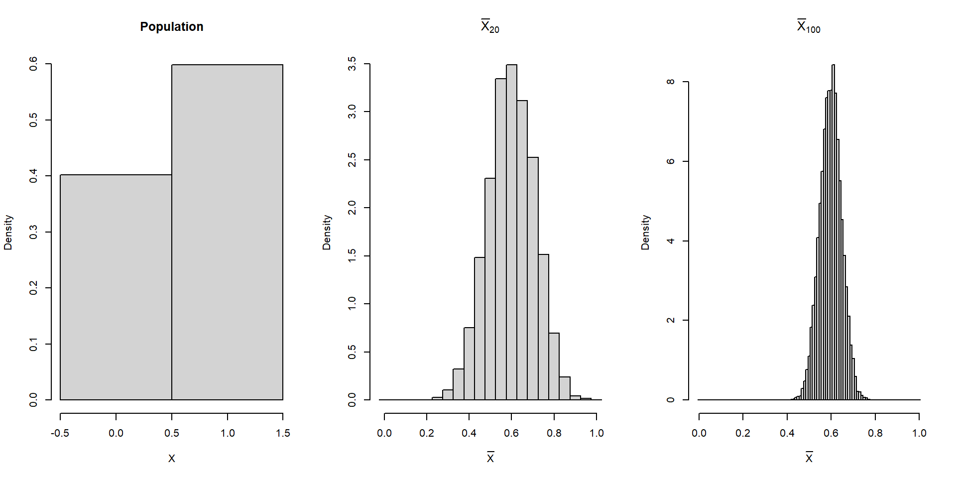
The population has only two possible values, but the sampling distribution of \(\bar X_n\) becomes approximately normal.
set.seed(20260709)

B <- 10000

# Population
x <- rbinom(100000, 1, p)

# Sampling distributions
xbar20 <- replicate(B, mean(rbinom(20, 1, p)))
xbar100 <- replicate(B, mean(rbinom(100, 1, p)))

par(mfrow = c(1,3))

hist(x,
     probability = TRUE,
     breaks = seq(-0.5,1.5,1),
     main = "Population",
     xlab = "X")

hist(xbar20,
     probability = TRUE,
     breaks = seq(-1/(2*20),1+1/(2*20),by=1/20),
     main = expression(bar(X)[20]),
     xlab = expression(bar(X)))

hist(xbar100,
     probability = TRUE,
     breaks = seq(-1/(2*100),1+1/(2*100),by=1/100),
     main = expression(bar(X)[100]),
     xlab = expression(bar(X)))